n-Dimensional Moving Least Squares projection

Background

Continuing with the theme of nD implementations of useful algorithms, here is my take on Moving Least Squares (MLS), a popular method used in engineering and graphics applications for smoothing out noisy point cloud data. Possibly data sources include laser scans, depth sensors (e.g. Kinect) or the like.

The basic principle of MLS projection is that you have a noisy point cloud approximating a surface. Projection means we’re going to take a point from anywhere in space and project it on this surface approximation. We will conveniently also get a surface normal for free as a result of doing this.

The Basic Algorithm

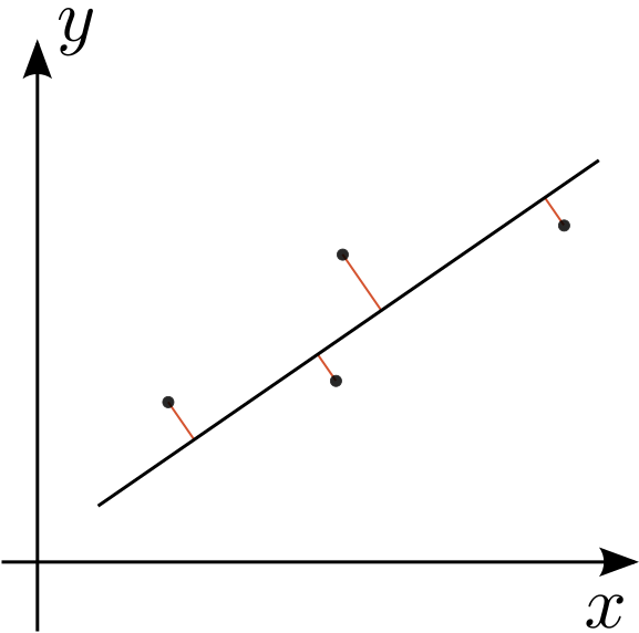
I’ll describe the projection algorithm with reference to the following figures:

We are given the original query site \\(q_0)\in\mathbb{R}^n\\) (the red point) and the existing point cloud consisting of points \\(x_i \in \mathbb{R}^n\\) (the black points) (note I'm going to use the indices of the query site and the point cloud differently - the index of \\(q\\) refers to the iteration number of the algorith, the index of \\(x\\) will refer to index of the nearby points). We are also given some query radius \\(r\\) which will contain all the points of interest. Note that the choice of \\(r\\) has a significant effect on the smoothness of the function - this will probably be a topic of discussion for a later post. In the images from right to left: 1. Identify all the points within the query radius \\(r\\) of \\(q_0\\), i.e. the set of points \\(\\{x_i : \\|x_i - q_0\\| < r\\}\\) 2. Construct a *best-fit plane* through these points by using a weighted least squares method (more on this later). Then *project* \\(q_0\\) onto this plane to find our next query point \\(q_1\\). 3. Iterate and continue until two consecutive steps of the projection result in very similar points, i.e. within some \\(\epsilon\\) which is some small error tolerance.

This is pretty trivially demonstrated using a code snippet from the implementation. In this example cpt is the current point (e.g. the iterating projected point \(q_j\)), tol is some user specified tolerance (equivalent to \(\epsilon\)). The rest should mostly be self-explanatory:

    // Continue this loop until we're close enough to the surface
    while (err > tol) {
        // Perform a least squares projection from the current point onto a best
        // fit hyperplane. The result will tell us if any neighbours were found.
        if (weightedLS(cpt, radius, plane, idxDist) == 0) {
            // What should we do here? throw an error?
            return cpt;
	}
        // If it all went well, we'll have a plane onto which the point can be projected
        tmp = plane.projection(cpt);

        // Our error is just the distance between the input point and our current point
        err = (tmp-cpt).norm();

        // Update our current point to the projected point
        cpt = tmp;
    }

    // If it all went well, we can assume our current point is the best one available
    return cpt;

Note that the function weightedLS() returns the number of points found within the query radius, and modifies the plane to contain the best fit plan through the points. If nothing was found within the radius there is a question of what you should do. Increasing the radius size is an obvious choice, but there may be continuity issues in the query data set.

Weighted Least Squares

So it is now important to drill down into the Weighted Least Squares fit function. There are some pretty useful references on everyones favourite academic source here. There is a much broader discussion here to be had about linear regression for fitting curves to polynomials, but I’ll restrict myself to the planar case.

The general implicit form for a plane $$\mathbf{n}\cdot(x - x_0)=0,$$ where \(\mathbf{n}\) is a normal to the plane (bold because it is a vector), and \(x_0\) is a point through which the plane passes. So the plane is defined by any point \(x\) for which the above function evaluates to exactly \(0\).

If the number of points is equal to the dimensionality the space it is easy enough to find the normal from the input points. For example, the normal to a vector $$ \mathbf{v}= \left[ \begin{array}\ x_1 - x_0 \\ y_1 - y_0 \end{array} \right] $$ between two points in \(\mathbb{R}^2\) is \((-v_y,v_x)\), for higher dimensions use the cross or wedge product.

As an aside, you might be interested to know that this can also be solved by solving for the null space of the system of equations given by \(\mathbf{n}\cdot(x - x_0)=0\) - recall that this system is underdetermined because one of the points provided will be \(x_0\). In \(\mathbb{R}^2\), this will be the equivalent of solving for the null space of $$ \begin{array}\
\mathbf{n} \cdot \mathbf{v} = 0\
n_x v_x + n_y v_y = 0 \end{array} $$ which is of course only non-trivially true when \(\mathbf{n} = (-\mathbf{v}_y,\mathbf{v}_x)\).

Note that we can also solve for the normal using the formula \(\mathbf{n}\cdot(x - x_0)=\alpha\) where \(\alpha\) is some arbitrary scalar as the normal is the same if we shifted it along the normal direction. This allows us to formulate the problem into a linear system $$X\textbf{n}=\textbf{b},$$ where \(X\) is the matrix of known points on the plane, \(\mathbf{n}\) is the unknown plane normal, and \(\mathbf{b}\) is some constant vector made up of \(\alpha\)’s. For simplicity let’s just let \(\alpha=1\) from now on. This is well defined if \(X\) is square, i.e. there are the same number of points as there are dimensions - this is because these points form a n-simplex in \(\mathbb{R}^n\).

Ok, now what happens if we have more points than dimensions? In this case, we can solve this in the least squares sense. This is essentially an optimisation problem, solved using the Moore-Penrose pseudoinverse. While there is buckets to write about this, it boils down to premultiplying both sides of the equation by \(X^T\) yielding $$X^T X \mathbf{n} = X^T \mathbf{b}.$$ Note that \(X^T X\) is now a square matrix, the system can be solved and has a unique solution. The solution itself is optimal in a least-squares sense, meaning that it minimizes the sum of the squares of the errors made in the results of each equation. Or put another way, it spreads the error love evenly between all of the point contributors to the plane.

Now applying weights to this should actually be quite straightforward: we’ll create some diagonal matrix of weights \(W\) where elements on the diagonal represent the amount we want to weight the error of each point in \(X\). So a smaller weight would mean that in a least squares sense we are consider the error to be less important. This is incorporated into the system above as follows: $$X^T W X \mathbf{n} = X^T W \mathbf{b}.$$ If we’re trying to write our plane equation as \(\mathbf{n}\cdot x = d\) where \(d\) is a constant, a property of the above process is that \(d=1 / |\mathbf{n}| \). Also you must still normalise the resultant normal, e.g. \(\mathbf{n} = \mathbf{n}d\). Note that this whole process works in any dimension - pretty neat.

There is also the small issue of how to decide on the weights. Any kernel function would do, and each will have an impact on the overall quality of the reconstruction. Currently I’m just inverting the distance, but this could lead to problems when the point is exactly on top of the query point. Other choices of kernel function, such as \(\exp({-s^2})\). Some experimentation depending on application will probably be required.

Here is the implementation of this in pointcloud.hpp:

    if (m_index.findNeighbors(results, pt.data(), nanoflann::SearchParams())) {
        // Weights matrix
        MatrixXr W(idxDist.size(), idxDist.size()); W.setZero();
        // The matrix of the actual points
        MatrixXr K(idxDist.size(), DIM);

        // The result of the call is true if a neighbour could be found
        typename ResultsVector::iterator it;
        int i,j;
        for (it = idxDist.begin(), i=0; it != idxDist.end(); ++it,++i) {
            // First check to see if this evaluates to 0 exactly (BAD)
            if ((*it).second == REAL(0)) {
                // Set the weight to half the max REAL value (risky)
                W(i,i) = std::numeric_limits<REAL>::max() * REAL(0.5);
            } else {
                // Set the weight to the inverse distance
                W(i,i) = 1.0 / (*it).second;
            }
            // Build the matrix K out of the point data
            for (j=0;j<DIM;++j) K(i,j) = m_data[(*it).first][j];
        }
        // Normalise the weights to make sure they sum to 1
        W = W / W.sum();

        // Now solve the system using the following formula from MATLAB
        // N' = (K'*diag(W)*K) \ (K')*diag(W)*(-ones(size(I,1),1));
        // d  = 1/norm(N);
        // N  = N' * d;
        VectorDr ans;
        MatrixXr A = K.transpose() * W * K;
        VectorDr b = -K.transpose() * W.diagonal();
        ans =  A.llt().solve(b);
        REAL d = REAL(1) / ans.norm();
        Hyperplane _h(ans * d, d);
        h = _h;

        // For the results structure to be useful we need it to store the weights from W, so
        // we copy these back into it
        for (it = idxDist.begin(), i=0; it != idxDist.end(); ++it,++i) {
            (*it).second = W(i,i);
        }
        // We return the number of effective matches
        return idxDist.size();
    } else {
        // No neighbours found! What do we do?
        return 0;
    }

The general dimensional hyperplane is managed by Eigen::Hyperplane which allows us to do projections (see previous code snippet). Note that the solver used is Eigen’s Cholesky solver, which is very fast by requires a matrix that is symmetric positive definite. Fortunately our matrix \(X^T W X\) has these properties. In practice it is very unwise to solve systems like \(A\textbf{x}=\textbf{b}\) by inverting \(A\).

Implementation details

The plan was to make this implementation general dimensional, and this has been achieved through liberal use of templates.

template <typename REAL, unsigned int DIM>
class PointCloud {

The top of our class says that we’re allowing you to choose your type to represent the data (called REAL) and the dimension of the data set, which can be anything you like. As mentioned previously, Eigen provides general dimensional hyperplane routines which makes our lives relatively simple.

Unfortunately as you may have realised from the above algorithm the performance is largely dependent on how quickly we can find all the points within a given radius. This is resolved using a KD tree, which essentially organises the points into a graph structure for fast searching. I’m not going to discuss the specifics of KD tree construction and querying - there are plenty of other links to help you with this. I chose to make use of nanoflann from Jose Luis Blanco-Claraco as it is a header only library making it easier to incorporate into the project build.

One issue which may seem non-obvious is that I have added the KD tree index object as a member of the PointCloud class:

    /// A KDTreeIndex type
    typedef nanoflann::KDTreeSingleIndexAdaptor<
        nanoflann::L2_Simple_Adaptor<REAL, PointCloud<REAL,DIM> > ,
        PointCloud<REAL,DIM>,
        DIM> KDTreeIndex;

    /// A KDTree structure
    KDTreeIndex m_index;

This means that the KDTreeIndex is incorporated into the PointCloud class, although as you can see from the typedef above the PointCloud is a template parameter for the index itself. This is because the class which is passed to nanoflann needs to have a set of functions (all with the prefix kdtree_) which will be called during kd tree construction and querying, for example:

    /// Returns the dim'th component of the idx'th point in the class (random point access)
    inline REAL kdtree_get_pt(const size_t idx, int dim) const {
        return m_data[idx][dim];
    }

The way this works is that we pass this object when we construct the KDTreeIndex, e.g.

/**
 * Build an empty point cloud with an empty KDTree.
 */
template <typename REAL, unsigned int DIM>
PointCloud<REAL,DIM>::PointCloud()
    : m_index(DIM, *this, nanoflann::KDTreeSingleIndexAdaptorParams(10)) {
}

It is an interesting and rather twisting compositional arrangement, but it allows us to make sure that all the elements relevent to the point cloud in one convenient place.

Another interesting trick of nanoflann compatibility is the fact that I’m storing my points in Eigen, while nanoflann needs to compute distances using data stored in pointers to REAL’s. Rather than constructing a new Eigen point and copy data across, we can make use of the Eigen::Map which will just make a vector out of the existing memory rather than copying it across, hopefully saving us a couple of clocks:

    /// Returns the distance between the vector "p1[0:size-1]" and the data point with index "idx_p2" stored in the class:
    inline REAL kdtree_distance(const REAL *p1_data, const size_t idx_p2, size_t size) const {
        Eigen::Map<const PointType> p1_map(p1_data,DIM);
        return (m_data[idx_p2] - p1_map).norm();
    }

Conclusions

Currently the examples of using this code are pretty spartan as it is going to be incorporate into a significantly larger project. However, there are a couple of important things to note about this implementation:

1. The choice of radius has a significant impact on the projection. In previous implementations I’ve geometrically scaled the radius until some points are found and then scaled it back after the first projection. However, this may have continuity implications. I’ve also used a precomputed smooth scalar field of radii to use for this projection to ensure that you have a constant number of neighbours - something I’ll be experimenting with in the future.
2. There are a couple of implementation issues I still need to resolve, such as the choice of weight function and how to handle the situation when there are no neighbours in the specificed radius (see above). There is also the relationship between the radius and the cell size of the KD Tree which needs to be resolved. And some nice 3D examples!
3. The process of using MLS projection to smooth input data (called mollification) was not discussed, but will hopefully be appended to this post at some point. The process is pretty simple: project each point in the existing set onto other points in the same set. This has some interesting performance considerations to doing it correctly (for example, the KD Tree will need to be rebuilt in each iteration).
4. Parallelism! There are a couple of things which could be done in parallel, especially if we’re doing mollification.

Downloads

The source code is hosted on GitHub. Clone it from the repository using the following command from your console:

git clone https://github.com/rsouthern/Examples