Lab 5 Introduction to Particle Systems
Aims
The aim of this lab is to develop a simple particle system and write data to various file formats. We will then visualize the data using 3rd party tools
- Introduction to Particle Systems
- Using std::vector
- Writing data to disk
- Visualizing data.
Introduction to Particle Systems
Particle systems were introduced in the 1983 paper Particle Systems—A Technique for Modeling a Class of Fuzzy Objects and can be seen in action in the “Genesis Effect” sequence from Star Trek II : The Wrath of Khan. It is interesting to note that this movie also has fractal terrain, alpha compositing and other core CGI elements that were basically invented for this sequence.
A particle system is usually generated as a collection of point like elements. Usually they are animated using a physics based system but using a simplified model. In most cases particles are assumed to not collide with themselves (to reduce complexity) and if rendering we make a number of assumptions to ensure rendering is quicker, for example lack of shadows etc.
Particle structure
Particle systems have changed very little from the days of the Original Reeves paper, where he proposed a Particle has the following basic attributes.
- initial position
- initial velocity (both speed and direction)
- initial size
- initial color
- initial transparency
- shape
- lifetime
Whilst not explicitly mentioned in the Reeves paper a particle system usually has a controlling class called the Emitter which acts as the source of the particle’s initial position. It will usually have methods to render and update the system as well as to add and remove particles.
classDiagram
class Vec3{
  x : float
  y : float
  z : float
}
class Particle{
  + pos : Vec3
  + dir : Vec3
  + colour : Vec3
  + life : int
  + size : float
}

class Emitter{
- m_particles : std::vector<Particle>
- m_position : Vec3
- m_spread : float
- m_emitDir : Vec3
+ Emitter(_pos : Vec3, _numParticles : size_t)
+ ~Emitter()
+ update()
+ saveFrame(_fname : const std::string &)
+ draw()
}

Emitter --> Vec3
Particle --> Vec3
Emitter "1" -->"1..*" Particle : Creates
System Outline
graph LR
A[Init<br>Emitter]-->B{Finished}
B -->|No|C[Update All<br>Particles]
C-->D[WriteFrame<BR>To File]
D-->B
B -->|YES| E[EXIT]
The overall simulation is quite simple, we will loop for each particle and update using a simple motion equation, we will then write the particle position and size to disk and update the simulation for the next frame. To start with we will do some simple updates to ensure the basic system works then we will add more elements to get a better system.
Getting Started.
We are going to use a combination of TDD an YAGNI techniques in developing this system. We are going to start by creating our empty project and tests as usual.
First we will create an empty project folder and add files as follows.
For ease I have created some starter boiler plate code for this. Download the file Particle.tgz and copy it to your labs folder.
To extract do the following.
tar vfxz Particle.tgz
mkdir Particle
cd Particle
mkdir src include tests
touch CMakeLists.txt
touch include/Particle.h
touch include/Emitter.h
touch include/Vec3.h
touch src/main.cpp
touch src/Emitter.cpp
touch tests/ParticleTests.cpp
We now add the following to CMakeLists.txt
# We will always try to use a version > 3.1 if avaliable
cmake_minimum_required(VERSION 3.2)

if(NOT DEFINED CMAKE_TOOLCHAIN_FILE AND DEFINED ENV{CMAKE_TOOLCHAIN_FILE})
   set(CMAKE_TOOLCHAIN_FILE $ENV{CMAKE_TOOLCHAIN_FILE})
endif()
# name of the project It is best to use something different from the exe name
project(Particle_build)
find_package(fmt CONFIG REQUIRED)

# Here we set the C++ standard to use
set(CMAKE_CXX_STANDARD 17)
# add include paths
include_directories(include)
# Now we add our target executable and the file it is built from.
add_executable(Particle)
target_sources(Particle PRIVATE src/main.cpp  src/Emitter.cpp  src/Vec3.cpp
include/Particle.h include/Emitter.h include/Vec3.h )
target_link_libraries(Particle PRIVATE  fmt::fmt-header-only)

#################################################################################
# Testing code
#################################################################################

find_package(GTest CONFIG REQUIRED)
include(GoogleTest)
enable_testing()
add_executable(ParticleTests)
target_sources(ParticleTests PRIVATE tests/ParticleTests.cpp  src/Emitter.cpp src/Vec3.cpp include/Emitter.h include/Particle.h include/Vec3.h)
target_link_libraries(ParticleTests PRIVATE GTest::gtest GTest::gtest_main )
gtest_discover_tests(ParticleTests)
And simple C++ files to test the build first main.cpp
#include <iostream>
#include <cstdlib>

int main()
{
  std::cout<<"Particle \n";
  return EXIT_SUCCESS;
}
and ParticleTests.cpp
#include <gtest/gtest.h>

TEST(Particle,ctor)
{
  ASSERT_TRUE(1==0);
}
TDD Steps
We will now start to generate our particle system bit by bit only developing the elements we need at the time. The rough order will be as follows
- Construct Particle with No attributes.
- Generate Default Vec3 class with x,y,z so we can add attributes to Particle
- Generate Particle struct with all attributes needed.
- Generate a Simple Emitter class with default Particles.
- Generate better initial particles (will require a new Random Class)
- Update the particles using algorithm outlined below.
- Write particles per frame to file.
- Play!
Particle Birth
To create the new particle the emitter will set the default values for a particle whilst adding some random variation.
p.pos = emitter position
p.dir = m_emitDir * randomPositiveFloat() + randomVectorOnSphere() * m_spread;
p.dir.m_y = std::abs(p.dir.m_y);
p.colour = randomPositiveVec3();
p.maxLife = randomPositiveFloat(5000)+500;
p.life = 0;
p.scale= 0.01f;
For ease we will use a simple random number generator class outlined here, however will will take a diversion for testing it. First we need to create the files
touch include/Random.h
touch src/Random.cpp
Then add
#ifndef RANDOM_H_
#define RANDOM_H_
#include "Vec3.h"
#include <random>

class Random
{
  public :
    static Vec3 randomVec3(float _mult=1.0f);
    static Vec3 randomPositiveVec3(float _mult=1.0f);
    static float randomFloat(float _mult=1.0f);
    static float randomPositiveFloat(float mult=1.0f);
    static Vec3 randomVectorOnSphere(float _radius=1.0f );

  private :
    static std::mt19937 m_generator;
};
#endif
#include "Random.h"
#include <cmath>
std::mt19937 Random::m_generator;

auto randomFloatDist=std::uniform_real_distribution<float>(-1.0f,1.0f);
auto randomPositiveFloatDist=std::uniform_real_distribution<float>(0.0f,1.0f);

Vec3 Random::randomVec3(float _mult)
{
  return Vec3(randomFloatDist(m_generator)*_mult,
              randomFloatDist(m_generator)*_mult,
              randomFloatDist(m_generator)*_mult);
}

Vec3 Random::randomPositiveVec3(float _mult)
{
  return Vec3(randomPositiveFloatDist(m_generator)*_mult,
              randomPositiveFloatDist(m_generator)*_mult,
              randomPositiveFloatDist(m_generator)*_mult);
}

float Random::randomFloat(float _mult)
{
  return randomFloatDist(m_generator)*_mult;
}
float Random::randomPositiveFloat(float _mult)
{
  return randomPositiveFloatDist(m_generator)*_mult;
}

Vec3 Random::randomVectorOnSphere(float _radius )
{
  float phi = randomPositiveFloat(static_cast<float>(M_PI * 2.0f));
  float costheta = randomFloat();
  float u =randomPositiveFloat();
  float theta = acos(costheta);
  float r = _radius * std::cbrt(u);
  return Vec3(r * sin(theta) * cos(phi),
              r * sin(theta) * sin(phi),
              r * cos(theta)
);

}
Finally don’t forget to add the source files to the CMakeLists for both targets.
When testing random number generators the best we can do is to test to see if multiple runs of the generator results in values within the range expected. For example randomPositiveFloat should only give positive values over a number of runs.
TEST(Random,positiveFloat)
{
  for(int i=0; i<100; ++i)
  {
    auto v=Random::randomPositiveFloat();
    EXPECT_TRUE(v>0.0f && v<=1.0f);
  }

  for(int i=0; i<100; ++i)
  {
    auto v=Random::randomPositiveFloat(20);
    EXPECT_TRUE(v>0.0f && v<=20.0f);
  }
}
Particle update algorithm
Each frame we will update the particle by using the following basic algorithm
dt = time step
gravity=Vec3(0.0f, -9.81f, 0.0f)
for each particle :
  dir += gravity * _dt * 0.5f
  pos += p.dir * _dt
  scale += randomPositiveFloat(0.05)
  life +=1
  if life >= maxLife or hit ground plane :
    resetParticle
This means that we now need to write operator overloads for the Vec3 class to allow us to add Vec3 elements.
Houdini geo format
No we have a basic working system we can start to write out the data into files each frame and load to Houdini to test.
The ASCII .geo and binary .bgeo file formats are the standard formats for storing Houdini geometry. The .geo format stores all the information contained in the Houdini geometry detail. To write out our particle system we only need a small section of the format to be filled in and it is quite simple.
Header Section
Magic Number: PGEOMETRY
Point/Prim Counts: NPoints # NPrims #
Group Counts: NPointGroups # NPrimGroups #
Attribute Counts: NPointAttrib # NVertexAttrib # NPrimAttrib # NAttrib #
In each of these cases, the # represents the number of the element described. Groups are named and may be defined to contain either points or primitives. Each point or primitive can be a member of any number of groups, thus membership is not exclusive to one group. In our case we will have _numParticles set for the value of NPoints and we are going to save two attributes of our particle system. The colour which Houdini will allocate if we set the Cd attribute and the scale which we will set to the houdini pscale attribute.
Attribute Definitions
Internally, there are “dictionaries” to define the attributes associated with each element. These dictionaries define the name of the attribute, the type of the attribute and the size of the attribute. Also, the default value of the attribute is stored in the dictionary.
Name Size Type Default
For our attributes we will write the following
NPointAttrib 2  NVertexAttrib 0 NPrimAttrib 1 NAttrib 0
PointAttrib
Cd 3 float 1 1 1
pscale 1 float 1
Finally the point data is written with the attributes as follows
x y z 1 ( Cd Cd Cd pscale)
^^^^^     ^^^^^^^^ ^^^^^^
position  Colour   scale
Finally we need to write out the index into the primitives list, with a full file of 10 particles at 0,0,0 with random colours shown.
PGEOMETRY V5
NPoints 10 NPrims 1
NPointGroups 0 NPrimGroups 0
NPointAttrib 2  NVertexAttrib 0 NPrimAttrib 1 NAttrib 0
PointAttrib
Cd 3 float 1 1 1
pscale 1 float 1
0 0 0 1 (0.826752 0.937736 0.746026 0.1)
0 0 0 1 (0.093763 0.623236 0.443004 0.1)
0 0 0 1 (0.941186 0.451678 0.684774 0.1)
0 0 0 1 (0.716227 0.405941 0.600561 0.1)
0 0 0 1 (0.918985 0.756861 0.584415 0.1)
0 0 0 1 (0.867986 0.576151 0.698259 0.1)
0 0 0 1 (0.215546 0.0504826 0.486265 0.1)
0 0 0 1 -0.936334 0.59456 0.412092 0.1)
0 0 0 1 (0.646916 0.988137 0.805736 0.1)
PrimitiveAttrib
generator 1 index 1 papi
Part 10 0 1 2 3 4 5 6 7 8 9 10 [0]
beginExtra
endExtra
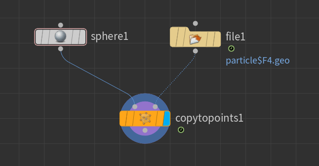
Loading into Houdini
As we have a size attribute saved as pscale we can use the copy to points node to scale a sphere for our visualization as shown.
Lets Play
Now we have a working system we can experiment and change things. One of the best ways of doing this is to create a git branch for each experiment. Assuming that the whole project is now under git version control we cna generate a new branch by doing the following.
git branch Experiment1
git checkout Experiment1
All changes to the project will now only be seen on the Experiment1 branch once commited. We can also push this to a different branch on GitHub by using the following.
git push -u origin Experiment1
And to change back to the master we use.
git checkout master
Things to try.
- In the original paper the generation of particles is done not all at once as we do now but using a distribution function where multiple particles are birthed each frame based on a random value. Update the emitter to try this.
- At present the particles have no Mass, using the equations of projectile motion update the simulation to add mass to the particles.
- At present we write to the Houdini Geo format, however there are other formats we can use. One easy way to do this is via the Disney partio library. Have a look and see how it can be used.