Compact Elliptical Basis Functions for Surface Reconstruction

\( \newcommand{\x}{\mathbf{x}} \newcommand{\n}{\mathbf{n}} \newcommand{\q}{\mathbf{q}} \newcommand{\e}{\mathbf{e}} \newcommand{\diag}{\mathsf{diag}} \newcommand{\khachiyan}{\mathsf{Khachiyan}} \newcommand{\flatClust}{\mathsf{flatClust}} \newcommand{\kmeans}{\mathit{k}\mathsf{means}} \newcommand{\sort}{\mathsf{sort}} \newcommand{\tP}{\tilde{P}} \newcommand{\idx}{\mathbf{i}} \newcommand{\tidx}{\tilde{\idx}} \newcommand{\List}{\mathcal{L}} \newcommand{\I}{\mathcal{I}} \newcommand{\eig}{\mathsf{eig}} \)

In this post I present a method to reconstruct a surface representation from a a set of EBF’s, and in addition present an efficient top-down method to build an EBF representation from a point cloud representation of a surface. I also discuss the advantages and disadvantages of this approach.

Radial basis functions (RBFs) are a popular variational representation of volumes and surfaces in computer graphics. In general, an RBF is a real-valued function whose value depends only on the distance from it’s center. A special class of these functions have compact support - in this case the function decays smoothly to zero as the radius approaches 1. In this way, only a relatively small number of RBF’s influence any particular point in space, which in turn greatly improves computational efficiency.

(a)	(b)
On certain features (a), basic radial basis functions are inefficient at capturing the surface properties. In comparison (b), very few elliptical functions would be needed to represent this feature.

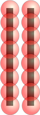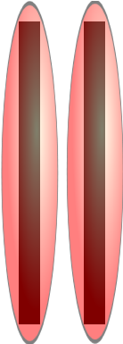However, certain features are not best represented by radial basis functions, such as in Figure below. Consider two parallel lines - if they are close enough together, you will need many RBF’s in order to ensure that the two features are separated. In comparison, an elliptical shape can better represent this structure (see figure).

In this technical report I present a method to reconstruct a surface representation from a a set of EBF’s, and in addition present an efficient top–down method to build an EBF representation from a point cloud representation of a surface. I also discuss the advantages and disadvantages of this approach.

Background

The reader is probably familiar with the well known general elliptical form \(x^2 / a^2 + y^2 / b^2 = 1\). This 2D formulation assumes the ellipse is centered at the origin, \(a\) and \(b\) are the lengths of the major and minor axes which are aligned with the Cartesian axes. In general we use the quadratic form for an ellipse \( Ax^2 + By^2 + Cx + Dy + Exy + F = 1 \). This can be rewritten in quadratic (matrix) form:

\begin{equation} f(\mathbf{x}) = (\mathbf{x}-\mathbf{q})^T Q (\mathbf{x}-\mathbf{q}) = 1 \label{eq:quadratic} \end{equation}

for ellipse center \(\mathbf{q}\) and shape matrix \(Q\). Note that for real roots, \(Q\) must be positive semi-definite, i.e. (\(Q = Q^T\) and \(\left\langle x, Qx \right\rangle \geq 0\) for all \(x\in\mathbb{R}^n\)). \(Q\) can be factorized into \(Q=M^TM\).

An alternative, more compact formulation is to use homogeneous coordinates \(\hat{\mathbf{x}} = \left[ \mathbf{x}, 1\right]^T\) and combine \(\mathbf{q}\) and \(Q\) into a single matrix with a translational component: \begin{equation} A = \left[ \begin{array}{cc} Q& 0\\
-\mathbf{q}& 1 \end{array} \right] \end{equation}

so that quadratic form becomes the homogeneous form for the ellipsoid. \begin{equation} f(\hat{\x}) = \hat{\x}^T A \hat{\x} = 1 \label{eq:homogeneous} \end{equation} In general we refer to the ellipse by the pair \([\q, Q]\). Note that the quadratic and homogeneous forms of the ellipsoid compute the elliptical radius. Note that the volume of an ellipse is given by \(v = \sqrt{\det(Q)}\).

Radial Basis Functions

Radial Basis Functions (RBF) provide a simple method to construct smooth implicit surfaces from data of arbitrary dimension. Given a matrix of sample points: \(P = \left[\x_1, \dots,\x_n \right]\) which we assume are generated by sampling on the smooth implicit surface \( \hat{f}(\mathbf{x}) = 0 \), we estimate this function using the a standard RBF formulation \begin{equation} f(\x) = \sum_{\q \in \mathcal{C}} \alpha_i \phi_{\sigma_i} \left(\left\|\x - \q\right\|\right) + \mathbf{b}^T p(\x), \label{eq:rbf} \end{equation} where \(\sigma\) is the local basis function radius for compactly supported RBFs \(\phi_{\sigma}(r) = \phi(r/\sigma)\), \(\phi(r)\) is a radial basis function, \(\mathbf{b}=[\beta_1,\ldots,\beta_{|p(\x)|}]^T\), \(\alpha_i\) and \(\beta_j\) are unknown coefficients and \(p(\x)\) is some polynomial in \(\x\) with \(|p(\x)|\) terms (A good choice for \(p(\x)\) is typically \(\x + 1\)). The set \(\mathcal{C}=\left\{\q_1,\ldots,\q_m\right\}\) contains the chosen (RBF) centers, and for a compact approximation we assume \(m \ll n\).

The choice of the basis function \(\phi(r)\) depends on the application - we have used globally supported spline \(\phi(r)=r^2 \log(r)\), near compactly supported Gaussian \(\phi(r)=e^{-r^2}\) and compactly supported Wendland functions [18] \begin{equation} \phi(r)=(1-r)^4_{+}(4r+1) \end{equation} Note, the \(f(r)_{+}\) operator ensures positivity, i.e. if \(f(r) \lt 0\) then \(f(r)_{+} = 0\), else \(f(r)_{+} = f(r)\).

Dinh and Turk [7] propose the use of the spline formulation of Chen and Suter [6] due to the ability to locally control the smoothness of the resulting surface. This formulation requires two additional smoothness parameters which must currently be chosen in an ad-hoc fashion. As we will define locally anisotropic basis functions, the derivation of locally adaptive variants of \(\phi\) adds an unnecessary layer of complexity that is best avoided.

Variational Implicit Surface Approximation

RBF’s have been used extensively for the interpolation of volumetric data, neural networks and smooth surface approximations [17,3]. For surface approximation, a subset of \(k\) input points are chosen as RBF centers are chosen from the input data \(\mathcal{C}_s\), and \(l\) additional centers are added which are known to be on the exterior of the object \(\mathcal{C}_e\), \(\mathcal{C}=\mathcal{C}_s \cup \mathcal{C}_e\).

We use the fact that

\begin{equation} f(\q) = \left\{ \begin{array}{rl} 0,& \q \in \mathcal{C}_s\\\\ -1,& \q \in \mathcal{C}_e \end{array} \right. \end{equation}

in order to evaluate the coefficients \(\alpha_i\) using linear regression. The problem can be stated in matrix form

\begin{equation} \left[ \begin{array}{cccc} \phi_{1,1}&\cdots&\phi_{1,m}&p(\q_1)\\\\ \vdots&\ddots&\vdots&\vdots\\\\ \phi_{m,1}&\cdots&\phi_{m,m}&p(\q_m)\\\\ p(\q_1)^T&\cdots&p(\q_m)^T&\mathbf{0} \end{array} \right] \left[ \begin{array}{c} \alpha_1\\\\ \vdots\\\\ \alpha_{k+l}\\\\ \mathbf{b} \end{array} \right] = \left[ \begin{array}{c} f(\q_1)\\\\ \vdots\\\\ f(\q_{k+l})\\\\ \mathbf{0} \end{array} \right], \end{equation}

where \(\phi_{i,j} = \phi_{\sigma_i}(\left|\q_i - \q_j\right|)\). Using the linear system above we can solve for the coefficients \(\alpha_i\) and \(\mathbf{b}\), and using these the implicit surface can be evaluated at any point using the RBF formulation.

Defining the locations of external centers \(\mathcal{C}_e\) requires some concept of the orientation of the surface. Often [14,15,17] an associated normal field is assumed. In these cases, an external center \(q_e\) is simply defined in terms of the center on the surface \(\q_s\), \(\q_e\) = \(\q_s\) + \(\psi \n_s\), for some \(\psi > 0\).

Elliptical basis functions

Anisotropic radial basis functions compute distances in the warped space, computed by applying the transformation matrix M.

The isotropic behavior of RBF interpolation and resulting smoothness is often not a desirable property. Consider the bunny’s ear in the figure. Because a single RBF center with a large \(\sigma_i\) is used to represent the flat part of the ear, the reconstruction does not reproduce this flat region. This problem could be solved by using many smaller centers to encode the flat region, but this can dramatically increase the size of the above linear system, making the problem expensive to solve.

For flat oriented regions an ellipse better approximates shape. Recall that the shape matrix ((Q\) describes the shape of the ellipse. In particular, because \(Q\) is positive semi-definite and symmetric, we can factorize it using singular value decomposition (in MATLAB, \([V, \lambda] = \eig(Q)\), \(M = V \diag(\sqrt{\lambda})V^T\)) to solve it \(Q=M^T M\). In this figure we warp the input space by transforming the input points using the ellipse shape matrix, i.e. \(\x' = M(\x-\q)+\q\). This space warping procedure is a method for local anisotropic interpolation.

Formulation

For an elliptical basis function formulation we define our set of centers as

\begin{equation} \mathcal{C}=\left\{[\q_1,Q_1,\sigma_1], \ldots, [\q_m,Q_m,\sigma_m]\right\}, \end{equation}

consisting of tuples containing the elliptical information. We can incorporate this local space warping matrix \(M\) in the RBF definition: \begin{equation} f_k(\x) = \sum_{\q \in \mathcal{C}} \alpha_{i,k} \phi_{\sigma_i} \left(\left|M_k (\x - \q)\right|\right) + \mathbf{b}_k^T p(\x). \end{equation} Note that we use a subscript \(k\) to denote which transformation function is used. The coefficients must now be computed for each EBF center (and hence each \(M_k\) using the linear system.

The problem of locally anisotropic RBF’s is resolved using a partition of unity approach. Loosely speaking, the coefficients \(\alpha_i\) and \(\beta_j\) are deduced for each of the elliptical centers \([\q,Q,\sigma]\in \mathcal{C}\). In order to evaluate an isovalue at some \(\x\), we compute a weight based on the proximity of \(\x\) from each center in the locally warped space. Then, the final isovalue is computed by computing the sum of these locally computed weighted functions.

More formally, we compute the isovalue by defining a new combined isosurface function \begin{equation} g(\x) = \frac{\sum_{k=1}^{m} w_k(\x) f_k(\x)}{\sum_{k=1}^{m} w_k(\x)} \label{eq:combined} \end{equation} with the isosurface at \(g(\x)=0\). By choosing a smooth weight function \(w_k(\x)\) we ensure that the reconstruction results of the combined isosurface function is also smooth. Casciola et al. [4] use the local weight function \begin{equation} w_k(\x) = \left(\frac{\left(\sigma_k - |M_k(\x - \q_k)|\right)_{+}}{\sigma_k |M_k(\x - \q_k)|}\right)^{\gamma_k}, \label{eq:weights} \end{equation} where \(\sigma_k\) is, the region of influence of each local anisotropic center and \(\gamma_k\) is a local regularization exponent. We have used \(\gamma_k=1\) for all our results. Note that \(\sigma_k\) here is used to both scale the radius in the EBF equation and to determine the weights, and is a measurement of the region of influence of a compact elliptical basis function.

So in summary, given a set of elliptical centers \(\mathcal{C}\) consisting of the position \(\q\), shape matrix \(Q\) and radius of influence \(\sigma\) of each center, we construct a variational implicit surface using elliptical basis functions as follows:

• For each center \([\q_k,Q_k,\sigma_k]\in\mathcal{C}\), compute the coefficients \(\alpha_{i,k}\), \(\mathbf{b}_k\) using the linear system as a preprocess.
• For an input point \(\x\), compute each of the weights \(w_k\).
• Compute \(g(\x)\) using these weights in using the EBF formulation and the combined isosurface function.

Building an EBF surface from point data

In this section we focus on the construction of EBF surfaces from point cloud data in any dimension without any shape information, such as surface normals. In order to construct an EBF surface we need a number of components:

• The elliptical shape properties of each center \(\q_k\) and \(Q_k\),
• The radius of influence of each center \(\sigma_k\),
• A normal field for the determination of external centers \(\mathcal{C}_e\), and
• Some radial basis function \(\phi(r)\).

For our application, we choose the radius of influence arbitrarily as the minimum radius needed to enclose a user specified number of neighboring centers in the warped elliptical space. For the radial basis function \(\phi(r)\) we make use of one of the standard RBF functions, depending on the application. In the following sections we will present a method for geometrically identifying the EBF centers and the the local region of influence for each center, as well as discuss our method to deduce the location and orientation of the elliptical centers.

Flatness clustering

Other authors have made use of either randomized [7] or bottom-up [4] approaches to selecting surface centers. Unfortunately these either yield unpredictable results, or are expensive because of the need to compute local curvature information at every input point.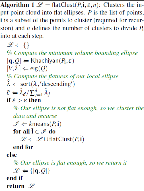

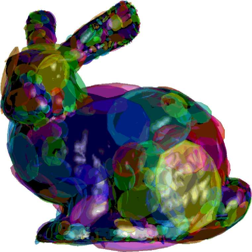
Constructing EBF's over a 3D point cloud.

We define a recursive top-down algorithm for partitioning an input set of points \(P\) into flat regions. Loosely speaking, we compute a minimum volume ellipse from the current list of points and measure the flatness. We measure the “flatness” by using the ratio of the minimum ellipse axis length over the sum of all elliptical axis lengths, similar to the the method of Luiz et al. [13]. If the surface is not sufficiently flat we subdivide the list of points by using a standard clustering algorithm, and append the results of recursive calls to the same function on each cluster.

The \(\flatClust\) algorithm makes use of the Khachiyan method for finding the minimum volume ellipse \(\khachiyan(P, \varepsilon)\), further discussed in the appendix. The eigenanalysis function \(\eig\) returns both the eigenvectors \(V\) and eigenvalues \(\lambda\). \(\kmeans(P,\idx)\) uses the method of Lloyd [12] to cluster only the points in \(P\) with the indices \(\idx\), and returns the set \(\I = \left\{ \tidx_1, \ldots, \tidx_n \right\}\) with each \(\tidx_j\) containing the indices of \(P\) belonging to each of the \(n\) clusters. We have used \(n=2\) for best results, although convergence is often faster when using a larger number of clusters. This approach can easily be applied to 3D data, as in the figure above.

Consistent orientation

In order to determine the external elliptical centers \(\mathcal{C}_e\) we require a local surface normal \(\n_s\). We can easily deduce an unoriented normal from the eigenvector of \(Q\) associated with it’s smallest eigenvalue.

A popular method for orienting these normals is by using the propagation method of Hoppe et al. [9]. In brief, this method constructs a Riemannian graph by defining each normal (tangent plane) as the nodes and edges connecting them are deduced using some proximity metric (in [9] this is the distance between the centers). A cost associated with an edge connecting node \(N_i\) to \(N_j\) is defined as \(1-|\n_i\cdot \n_j|\). The tree is traversed with a minimal spanning tree [16]. Whenever an edge \((i,j)\) is traversed, the orientation of \(\n_i\) is corrected if \(\n_i \cdot \hat{\n}_j \lt 0\), where \(\hat{\n}\) has already been corrected.

In order to approximate the Riemannian graph, and thereby reduce the computation time and errors arising from using a minimal spanning tree, we instead determine neighboring centers by using ellipse intersection. Traditional ellipse intersection techniques require computing the roots of a quadratic polynomial, which can be time-consuming to compute numerically.

Alfano and Greer [1] present a method to test for the intersection of two ellipses \(A\) and \(B\) (in the homogeneous form). The roots of the intersection can be found by determining \([V,\lambda] = \eig(A^{-1} B)\) and testing eigenvectors associated with non-real or repeated eigenvalues. This approach is easy to implement and very efficient as \(A^{-1}\) can be precomputed for all ellipses.

Consolidation

Because \(\kmeans\) clustering is not flatness sensitive, flat regions may become fragmented due to this procedure. An additional consolidation step is required to merge neighboring elliptical centers which exhibit the same flatness. We deduce the neighborhood of each ellipse by using the same intersection method described in the section above, and use a simple bottom-up method to combine elliptical centers the elliptical error given by \begin{equation} \tilde{\varepsilon} = \frac{\hat{\lambda}_d}{\sum_{j=1}^{d} \hat{\lambda}_j} \end{equation} is less than some user specified tolerance \(\varepsilon\).

Results

I have applied this method reconstruct the curve silhouette of the bunny model from sample points in 2D. As the compact RBF representation gradually transforms into an EBF representation, the contours sharpens - the best result probably is given in (c). However, note that as the ellipse thins, the internal and external contours deteriate, potentially leading to unpleasant numerical artefacts.

(a)	(b)	(c)
(d)	(e)	(f)
Gradually transforming the compact EBF shape matrices from radial (RBF) to elliptical. From (a) to (c), the sharpening of the resulting contour is clearly visible at the bunny foot. The shape contour begins to deteriorate in (d) to (e), as ellipses that are orthogonal to the surface begin influencing the interior of the shape. In this example, sigma is chosen to include the 10 nearest centers.

Conclusion

In this technical report I have demonstrated a method to build and represent point set surfaces using a scattered data interpolation technique based on compactly supported elliptical basis functions (EBF’s). While the technique has been successfully employed elsewhere in representing volume (and image) data, it’s application to surfaces is largely unexplored.

While this initial finding does show promise, my suspicion is that this approach has a number of considerable failings:

• Computation: It is computationally very expensive to solve the variational system for every elliptical basis function - which is the reason for no 3D results being included in this report. I believe that one possible option is to significantly improve the performance of the interpolation if only a limited subset of EBF’s are used to represent a shape, in the same way that a Gabor Wavelet filter bank has a limited number of filter orientations. In fact, an interesting idea for future work is to deduce an algorithm that adaptively determines the best orientations of a limited number of EBF’s in order to represent the shape.
• Accuracy: While some of the shapes in the results are promising, I am very concerned about the bottom row - as the EBF thins, the shape of the contour deteriorates significantly, which may cause numerical instabilities when the EBF’s are not chosen correctly. How to fit EBF’s to a surface without excessive thinning is a difficult problem, and certainly not addressed here.

Appendix: Minimum Volume Enclosing Ellipse

Given \(n\) points \(\x_i,,i=1,\ldots,n\), find the minimum volume enclosing ellipsoid. This is effectively the optimization problem \([\min \left[\log\left(\det(Q)\right)\right],,\mathrm{s.t.},,(\x_i - \q)^T Q (\x_i - \q) \leq 1.\)

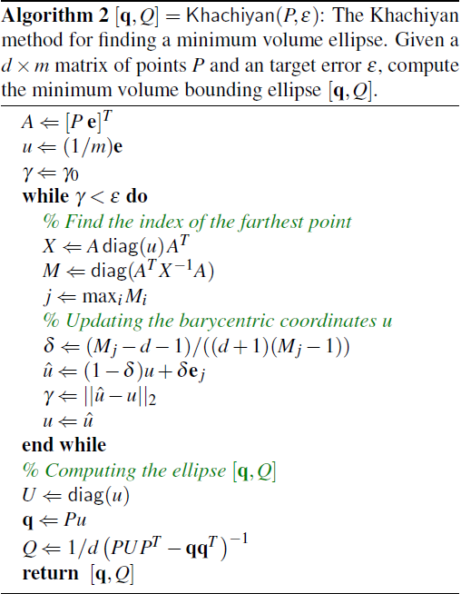
This problem is solved using the Khachiyan method [11], also known as barycentric coordinate ascent. This approach finds the barycentric coordinates \(u\) of a center of the ellipse in terms of the input points \(P\) by an iterative algorithm which shifts \(u\) closer to the farthest point from the center \(\q=Pu\). The optimal step-size \(\delta\) is deduced using the method presented by Kachiyan [11]. In the algorithm, \(\e\) is an \(m\)-length vector of ones and \(\e_j\) is the \(j_{th}\) basis vector. This method is typically greatly accelerated by using only the points on the convex hull of \(P\). For this we use the QHull method [2].

References

[1] Salvatore Alfano and Meredith L. Greer. Determining if two solid ellipsoids intersect. Journal of Guidance, Control, and Dynamics, 26(1):106–110, 2003.

[2] C.B. Barber, D.P. Dobkin, and H.T. Huhdanpaa. The quickhull algorithm for convex hulls. ACM Trans. on Mathematical Software, 22(4):469–483, December 1996. http://www.qhull.org.

[3] J. C. Carr, R. K. Beatson, J. B. Cherrie, T. J. Mitchell,W. R. Fright, B. C. McCallum, and T. R. Evans. Reconstruction and representation of 3d objects with radial basis functions. In SIGGRAPH ’01: Proceedings of the 28th annual conference on Computer graphics and interactive techniques, pages 67–76, New York, NY, USA, 2001. ACM. ISBN 1-58113-374-X.

[4] G. Casciola, D. Lazzaro, L. B. Montefusco, and S. Morigi. Shape preserving surface reconstruction using locally anisotropic radial basis function interpolants. Comput. Math. Appl., 51(8):1185–1198, 2006. ISSN 0898-1221. doi: http://dx.doi.org/10.1016/j.camwa.2006.04.002.

[5] G. Casciola, L. B. Montefusco, and S. Morigi. Edge-driven image interpolation using adaptive anisotropic radial basis functions. J. Math. Imaging Vis., 36(2):125–139, 2010. ISSN 0924-9907. doi: http://dx.doi.org/10.1007/s10851-009-0176-8.

[6] F. Chen and D. Suter. Multiple order laplacian spline — including splines with tension. Technical Report MECSE 1996–5, Dept. of Electrical and Computer Systems Engineering, Monash University, July 1996.

[7] Huong Quynh Dinh and Greg Turk. Reconstructing surfaces using anisotropic basis functions. In International Conference on Computer Vision (ICCV) 2001, pages 606–613, 2001.

[8] Wei Hong, Neophytos Neophytou, Klaus Mueller, and Arie Kaufman. Constructing 3d elliptical gaussians for irregular data. In Mathematical Foundations of Scientific Visualization, Comp. Graphics, and Massive Data Exploration. Springer-Verlag, 2006.

[9] Hugues Hoppe, Tony DeRose, Tom Duchamp, John McDonald, and Werner Stuetzle. Surface reconstruction from unorganized points. In SIGGRAPH ’92: Proceedings of the 19th annual conference on Computer graphics and interactive techniques, pages 71–78, New York, NY, USA, 1992. ACM. ISBN 0-89791-479-1. doi: http://doi.acm.org/10.1145/133994.134011.

[10] Y. Jang, R. P. Botchen, A. Lauser, D. S. Ebert, K. P. Gaither, and T. Ertl. Enhancing the interactive visualization of procedurally encoded multi–field data with ellipsoidal basis functions. Computer Graphics Forum (Proceedings of Eurographics), 3(25), 2006.

[11] Leonid G. Khachiyan. Rounding of polytopes in the real number model of computation. Mathematics of Operations Research, 21(2):307–320, May 1996.

[12] S. P. Lloyd. Least square quantization in PCM. IEEE Transactions on Information Theory, 28(2): 129–137, 1982.

[13] Boris Mederos Luiz, Luiz Velho, Luiz Henrique, and De Figueiredo. Moving least squares multiresolution surface approximation. In Brazilian Symposium on Computer Graphics and Image Processing SIBGRAPI, 2003.

[14] Y. Ohtake, A. Belyaev, M. Alexa, G. Turk, and H. Seidel. Multi-level partition of unity implicits. In Proceedings of SIGGRAPH, pages 463–470, 2003.

[15] Y. Ohtake, A. Belyaev, and H. Seidel. 3d scattered data approximation with adaptive compactly supported radial basis functions. In Conf. Shape Modeling and Applications, pages 31–39, 2004.

[16] R. C. Prim. Shortest connection networks and some generalizations. Bell System Technical Journal, 36(1):1389–1401, 1957.

[17] G. Turk and J. F. O’Brien. Variational implicit surfaces. Technical Report GIT- GVU-99-15, Georgia Institute of Technology, 1999.

[18] H.Wendland. Piecewise polynomial, positive definite and compactly supported radial basis functions of minimal degree. In Advances in Computational Mathematics 4, pages 389–396, 1995.